On the Verification of Weighted Kripke Structures Under Uncertainty
Authors: Giovanni Bacci, Mikkel Hansen and, Kim G. Larsen
Affiliation: Department of Computer Science, Aalborg University, Denmark
e-mail: {giovbacci,mhan,kgl}@cs.aau.dk
We considered the problem of checking weighted CTL properties for weighted Kripke structures in presence of imprecise weights. We consider two extensions of the notion of weighted Kripke structures, namely (i) parametric weighted Kripke structures, having transitions weights modelled as affine maps over a set of parameters and, (ii) weight-uncertain Kripke structures, having transition labelled by real-valued random variables as opposed to precise real valued weights.
Utilities
Quantifier elimination for the theory of linear arithmetic
In this tutorial we will use quantifier elimination for checking the robustness of a WKS when uncertainties on its weights are quantified by means of an absolute error. Mathematica implements a built-in quantifier elimination algorithm, however if one needs a more efficient method one could use Mjollnir.
Mjollnir is a tool developed by David Monniaux that implements quantifier elimination algorithm for the theory of linear real arithmetic. The tool is freely available at http://www-verimag.imag.fr/~monniaux/download/Mjollnir_2012-02-24.zip
Once installed you shall set the installation directory as done below.
Test
By default, quantifier elimination is performed using Mjollnir. Run the following test to check if Mjollnir works correctly.
![]()
![]()
In case the test does not work you can set the Method as Automatic and use Resolve
![]()
![]()
Weighted Kripke Structures Utilities
The following function displays models. The function requires one to install Graphviz and the PVTool2. Once installed you shall set the installation directories as done below.
Sample WKSs from a given WUKS. The models will be saved in different files within the selected destination directory path
Model checking Weighted Kripke Structures under Uncertainties
Model Checking Parametric Weighted Kripke Structures
Interpret the output of the tool
Parse the output from the PVtool
![]()
Partial Evaluation of the parsed output
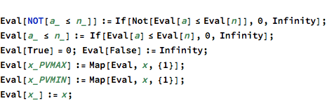
Encode the numerical formula as an first-order logic formula in the existential (linear) real theory of the reals.
Model Checking pWKS against bounded-WCTL
Compute the least fixed point of the EPDG associated with the pWKS P, state s, and the bounded WCTL formula phi. The function requires one to have installed Graphviz and the PVTool2. Once installed you shall set the installation directories as done below.
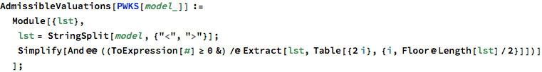
Symbolic representation of the set of evaluations solving the model checking problem

Symbolic representation of the admissible valuations
Example
![]()
![]()
![]()
![]()
![]()
![]()
Probabilistic Model Checking of Weight-Uncertain Kripke Structures
Monte Carlo Estimation
Number of samples based on the Chernoff bound
![]()
Estimate the event by sampling the random variables
Model Checking WUKS against bounded-WCTL
Example
![]()
![]()
Examples
Lawn Mower Example
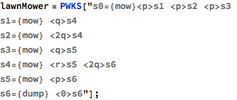
Consider the PWKS below representing a grass field with different routes a lawn mower can take from the starting state s0 to s6 where the grass can be dumped. The weights on the transitions represent the amount of grass that is accumulated in the container when selecting a particular route.
![]()
Assume that the lawn mower breaks when it is forced to store more than 6.5 units of grass, then the property “the grass is always dumped before the lawn mower breaks, irrelevant of the selected route” is expressed by the WCTL formula φ = ∀(mow ![]() dump).
dump).
![]()
To model check the PWKS lawnMower against φ, we can invoke the PVTool. The PVTool will construct an Extended Parametric Dependency Graph (EPGD) and symbolically compute its least fixed point assignment associated to the root configuration <s0, φ>.
Optionally, one can visualise the EPDG by setting the “EPDG” option to True (by default the option is disabled).
![]()
![]()
The set of admissible valuations for the lawnMower model can be retrieved as follows
![]()
![]()
The set of valuations satisfying φ, i.e., [[lawnMower, s0 |= φ]], can be represented by the following linear constraints
![]()
![]()
Assume that we have measured p = 2 ± ε, q = 1 ± ε and r = 0 ± ε where ε represents the the absolute measurement error of our parameters. One can determine if the model is robust with respect to φ by checking that all possible measurements values lay in [[lawnMower, s0 |= φ]].
This can be expressed by the following first-order formula in the theory of real linear arithmetic
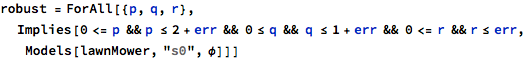
![]()
we can eliminate the quantifiers and obtain an equivalent formula
![]()
![]()
The above formula indicates that to ensure robustness, the error ε shall not exceed 1/10.
Assume now that the measurements for p, q and, r are associated to a distribution, i.e., they are modelled as real-valued random variables. The lawnMower shall be now modelled as a Weight-Uncertain Kripke Structure (WUKS).
Consider for instance that p~N(2,ε), q~Unif(1-ε,1+ε) and, r~N(0,ε) where ε= 1/10. We can declare the corresponding WUKS, called uncLawnMower, as follows
![]()
Note that the tool supports any of the distributions provided by Mathematica (cf. Random Variables).
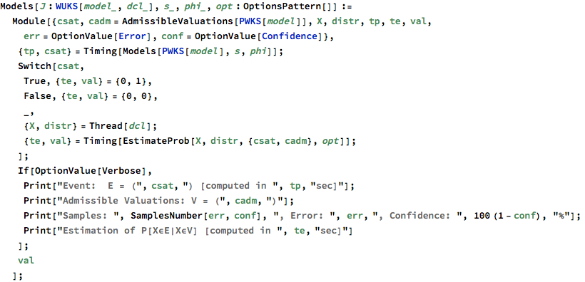
Now we can estimate the probability that uncLawnMower satisfies φ as follows. In this example we have set the error and the confidence for the estimation respectively to 0.005 and 0.001 by setting the options Error and Confidence (default values are Error → 0.005 Confidence → 0.0001). Futhermore one can set the option Verbose to True to printout some information regarding the estimation.
![]()
![]()
![]()
![]()
![]()
![]()
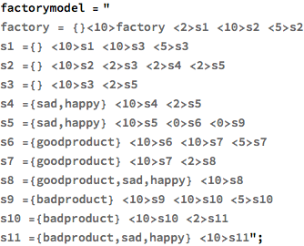
Factory Example
![]()
![]()
![]()