The CTMC-Dist Mathematica package
On-the-fly computation of bisimilarity distances for Continuous-Time Markov Chains
Authors: Giorgio Bacci, Giovanni Bacci, Kim G. Larsen, and Radu Mardare
The following tutorial aims at presenting the main features of the CTMCDist package. This Mathematica package implements three different methods for computing the bisimilarity distance between continuous-time Markov Chains (CTMCs):
iterative method;
linear programming method;
on-the-fly method.
Further details about their implementations can be found in a related technical-report paper ![]() .
.
The current package extends the BisimDist Mathematica library ![]() to continuous-time Markov chains, and is inspired from prevoius work on bisimilarity distances on Markov chains
to continuous-time Markov chains, and is inspired from prevoius work on bisimilarity distances on Markov chains ![]()
![]() .
.
Preliminaries
Continuous-Time Markov Chains and Stochastic Bisimilarity
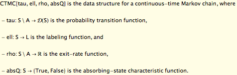
Definition (Continuous-time Markov chain). An L-labelled continuous-time Markov chain (CTMC) is a tuple M = (S, A, τ, ρ, ℓ) consisting of a nonempty finite set S of states, a set A ⊆ S of absorbing states, a transition probability function τ : S\A → D(S) (where D(S) is the set of probability distributions over S), an exit-rate function ρ : S\A → ![]() , and a labelling function ℓ : S → L.
, and a labelling function ℓ : S → L.
The labels L represent properties of interest that hold in a partucular state according to the labelling function ℓ. If s ∈ S is the current state of the system and E ⊆ S is a subset of states, τ(s)(E) ∈ [0,1] corresponds to the probability that a transition from s to arbitrary s’∈ E is taken, and ρ(s) ∈ ![]() represents the rate of an exponentially distributed random variable that characterizes the residence time in the state s before any transition is taken. Therefore, the probability to make a transition from stete s to s’∈ E within time unit t∈
represents the rate of an exponentially distributed random variable that characterizes the residence time in the state s before any transition is taken. Therefore, the probability to make a transition from stete s to s’∈ E within time unit t∈ ![]() is given by τ(s)(E) ·
is given by τ(s)(E) ·![]() for any Borel subset E ⊆
for any Borel subset E ⊆ ![]() .
.
Definition (Stochastic Bisimulation). Let M = (S, A, τ, ρ, ℓ) be an CTMC. An equivalence relation R ⊆ S × S is a stochastic bisimulation on M if whenever (s,t) ∈ R, then the following hold
ℓ(s) = ℓ(t);
s ∈ A iff t ∈ A;
if s,t ∉ A then ρ(s) = ρ(t) and, for all R-equivalence class C, τ(s)(C) = τ(t)(C).
Intuitively, two states are bisimilar if they have the same labels, they agree on being absorbing or not, and, in the case they are non-absorbing, their residence-time distributions and probability of moving by a single transition to any given class of bisimilar states is always the same.
Two states s,t ∈ S are bisimilar with respect to M, written s ∼ t, if they are related by some stochastic bisimulation on M.
Bisimilarity Pseudometric
Following the approach of ![]() , given a CTMC M = (S, A, τ, ρ, ℓ) we define 1-bounded pseudometric on S as the least fixed point of an operator on the set S × S → [0,1]. This pseudometric is then shown to be adequate with respect to stochastic bisimilarity: it has been proved that two states are stochastic bisimilar if and only if they have distance zero.
, given a CTMC M = (S, A, τ, ρ, ℓ) we define 1-bounded pseudometric on S as the least fixed point of an operator on the set S × S → [0,1]. This pseudometric is then shown to be adequate with respect to stochastic bisimilarity: it has been proved that two states are stochastic bisimilar if and only if they have distance zero.
The operator uses three key ingredients. The first one is a 1-bounded metric on the set of labels
![]()
a distance between residence-time distributions, and a distance beween transition ditributions. The first is meant to measure the static differences with respect to the labels associated with the states, the last two are meant to capture the differences in the dynamics, respectively, with respect to the continuous and discrete probabilistic choices.
To this end, we consider two distances over probability distributions. The first one is the so called total variation metric, defined for arbitrary distributions, μ,ν ∈ D(![]() ) as
) as
![]()
where the supremum is taken over the Borel measurable sets of ![]() . The second one is the Kantorovich distance, that for arbitrary distributions μ,ν ∈ D(S) is defined as
. The second one is the Kantorovich distance, that for arbitrary distributions μ,ν ∈ D(S) is defined as
![]()
Intuitively, ![]() lifts a (1-bounded) distance over S to a (1-bounded) distance over probability distributions. One can show that
lifts a (1-bounded) distance over S to a (1-bounded) distance over probability distributions. One can show that ![]() is a (pseudo)metric if d is a (pseudo)metric.
is a (pseudo)metric if d is a (pseudo)metric.
Now, we consider the following functional operator from which we will induce the bisimilarity distance
Definition. Let M = (S, A, τ, ρ, ℓ) be an CTMC and λ ∈ (0,1) a discount factor. The λ-discounted bisimilarity pseudometric for M, written ![]() , is the least fixed point of the function
, is the least fixed point of the function ![]() : (S × S → [0,1]) → (S × S → [0,1]), defined, for d : S × S → [0,1] and s,t ∈ S, as
: (S × S → [0,1]) → (S × S → [0,1]), defined, for d : S × S → [0,1] and s,t ∈ S, as
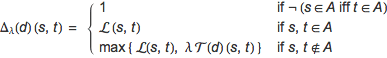
where T : (S × S → [0,1]) → (S × S → [0,1]) and L, E : S × S → [0,1] are respectively defined as
![]()
![]()
![]()
The functional ![]() measures the differences of two states with respect to: their labels (by means of the pseudometric L), their residence-time distributions (by means of the pseudometric E), and their discrete probabilities to move to the next state (by means of the Kantorovich distance). If two states disagree on been absorbing (or not) they are considered incompatible, and their distance is set to 1. If both states are absorbing, they express no dynamic behavior, hence they are compared statically, and their distance corresponds to that occurring between their respective labels. Finally, if the states are non-absorbing, then they are compared with respect to both their static and dynamic features, namely, taking the maximum among their respective associated distances.
measures the differences of two states with respect to: their labels (by means of the pseudometric L), their residence-time distributions (by means of the pseudometric E), and their discrete probabilities to move to the next state (by means of the Kantorovich distance). If two states disagree on been absorbing (or not) they are considered incompatible, and their distance is set to 1. If both states are absorbing, they express no dynamic behavior, hence they are compared statically, and their distance corresponds to that occurring between their respective labels. Finally, if the states are non-absorbing, then they are compared with respect to both their static and dynamic features, namely, taking the maximum among their respective associated distances.
It has been shown that ![]() for arbitrary discount factors, is adequate with respect to stochastic bisimilarity, that is
for arbitrary discount factors, is adequate with respect to stochastic bisimilarity, that is ![]() (s,t) = 0 if and only if s and t are stochastic bisimilar, s ∼ t.
(s,t) = 0 if and only if s and t are stochastic bisimilar, s ∼ t.
Loading the package
The package can be loaded by setting the current directory to that of the CTMCDist package and then using the commad << (Get) as follows. Here we use the directory of the current Mathematica notebook, referred by NotebookDirectory.
![]()
Encoding Continuous-Time Markov Chains
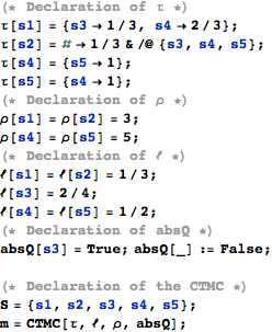
A CTMC M = (S, A, τ, ρ, ℓ) with ![]() is represented by a term of the form CTMC[τ,ℓ,ρ,absQ]
is represented by a term of the form CTMC[τ,ℓ,ρ,absQ]
![]()
The set of states ![]() can be represented symbolically; a probability distribution D(S) is encoded as a list of rules
can be represented symbolically; a probability distribution D(S) is encoded as a list of rules ![]() , where
, where ![]() is the probability associated with
is the probability associated with ![]() ; and absQ represent the characteristic function such that absQ[
; and absQ represent the characteristic function such that absQ[![]() ] iff
] iff ![]() ∈ A.
∈ A.
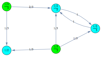
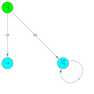
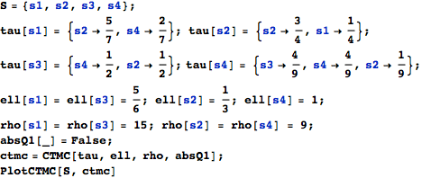
For example we can encode a CTMC m by defining τ,ρ,ℓ, and absQ, as follows:
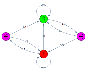
The CTMC m can is displayed by means of its undelying graph. Different labels are associated with different colors.
![]()
![]()
![]()
Computing the behavioral distance ![]()
On-the-fly method
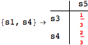
Given a CTMC m, a discount factor λ ∈ (0,1), and a list of pairs of states Q, one can compute the bisimilarity distance between the pairs listed in Q by calling the function BDistCTMC as follows
![]()
![]()
The Verbose option may be used to trace the computation steps
![]()
![]()
![]()
![]()
![]()
![]()
![]()
![]()
![]()
![]()
![]()
![]()
![]()
![]()
![]()
![]()
![]()
![]()
![]()
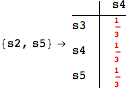
For computing the distance between all pair of states one can use as query list AllPairs[S]
![]()

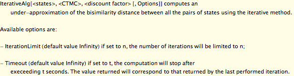
Iterative method
A second approach to compute the bisimilarity distance is given by computing an under-approximation by iterating the operator ![]() a number of times. To this end, the CTMCDist package provides the function IterativeAlg
a number of times. To this end, the CTMCDist package provides the function IterativeAlg
![]()
for example, we can compute the 10th iterate of ![]() by executing the following expression. One can set the number of performed iterations using the option IterationLimit
by executing the following expression. One can set the number of performed iterations using the option IterationLimit
![]()

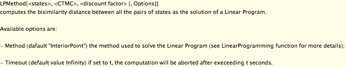
Linear Programming method
The third approach for computing the bisimilarity distance consists in solving the linear program that characterizes the distance.
The CTMCDist package provides the function LPMethod that generates the LP program and uses the built-in funtion LinearProgramming
![]()
![]()

![]()

Bisimilarity Distance and Bisimilarity Quotient
Due to the fact that ![]() (s,t) equals zero if and only if the states s and t are bisimilar,
(s,t) equals zero if and only if the states s and t are bisimilar, ![]() can be used to compute the bisimilarity classes and the bisimilarity quotient for a given CTMC.
can be used to compute the bisimilarity classes and the bisimilarity quotient for a given CTMC.
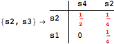
The CTMCDist package provides the functions BisimClassesCTMC and BisimQuotientCTMC that respectively computes the bisimilarity classes and the bisimilarity quotient of a given CTMC.
![]()
![]()
![]()
For example, using the function BisimClassesCTMC one can compute the bisimilarity classes of the CTMC m.
![]()
![]()
here we can see that ![]() ∼
∼ ![]() and
and ![]() ∼
∼ ![]() . Therefore we can lump together bisimilar states obtaining a minimized version of the CTMC that is behaviorally equivalent to m. This can be done using the function BisimQuotientCTMC as follows.
. Therefore we can lump together bisimilar states obtaining a minimized version of the CTMC that is behaviorally equivalent to m. This can be done using the function BisimQuotientCTMC as follows.
![]()
Examples
Example 1
Here we repropose Example 5.1 form![]() .
.
Let us compute the undiscouted distance between the state ![]() and
and ![]() , namely
, namely ![]()
![]()
![]()
![]()
![]()
![]()
![]()
![]()
![]()
![]()
![]()
![]()
![]()
![]()
![]()
![]()
![]()
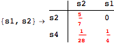
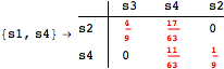
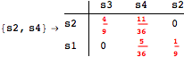
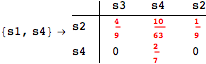
Looking at the execution trace we see that during the computation of d(s1,s4) an over-approximation for the distance beween the pairs {(s1,s2),(s1,s4),(s2,s3),(s2,s4)} is demanded. Since, the λ-discrepancy for (s2, s3), (s2, s4), and (s1, s2) equals the distance L between their labels, it coincides with the bisimilarity distance, hence it cannot be further decreased. Consequently, those values will be stored and successively used to cut further the searching space.
This can be seen in the second coupling structure, where only the input pair is demanded for computing the associated λ-discrepancy.
The following execution trace shows that the exact computation of ![]() demands for the pairs {(s1,s2),(s1,s4),(s2,s3),(s2,s4)} as in the previous example. Here insted we immediately note that the λ-discrepancy for (s2, s4) equals the distance L between their labels, therefore, we can terminate the computation even before checking for some other coupling structures.
demands for the pairs {(s1,s2),(s1,s4),(s2,s3),(s2,s4)} as in the previous example. Here insted we immediately note that the λ-discrepancy for (s2, s4) equals the distance L between their labels, therefore, we can terminate the computation even before checking for some other coupling structures.
![]()
![]()
![]()
![]()
![]()


![]()
![]()
![]()
![]()
![]()
![]()
Bibliography
1 Giorgio Bacci, Giovanni Bacci, Kim G. Larsen, and Radu Mardare. On-the-fly computation of Bisimilarity Distances. Submitted to LMCS for the special issue of TACAS 2013.
2 Giorgio Bacci, Giovanni Bacci, Kim G. Larsen, and Radu Mardare. The BisimDist Library: Efficient Computation of Bisimilarity Distances for Markovian Models.
In QEST 2013, volume 8054 of LNCS, pages 278-281, Springer Berlin Heidelberg, 2013.
3 Di Chen, Franck van Breugel, and James Worrell. On the Complexity of Computing Probabilistic Bisimilarity. In FoSSaCS 2012, volume 7213 of LNCS, pages 437–451. Springer, 2012.
4 Giorgio Bacci, Giovanni Bacci, Kim G. Larsen, and Radu Mardare. On-the-Fly Exact Computation of Bisimilarity Distances. In TACAS, volume 7795 of Lecture Notes in Computer Science, pages 1–15, 2013.
5 Franck van Breugel, Claudio Hermida, Michael Makkai, and James Worrell. Recursively defined metric spaces without contraction. Theoretical Computer Science, 380(1-2):143–163, 2007
6 Giorgio Bacci, Giovanni Bacci, Kim G. Larsen, and Radu Mardare. On-the-fly computation of Bisimilarity Distances. Submitted to LMCS for the special issue of TACAS 2013.