On-the-Fly Exact Computation of Bisimilarity Distances
Tutorial for the prototype implementation
Authors: Giorgio Bacci, Giovanni Bacci, Kim G. Larsen, and Radu Mardare
This is a tutorial for the prototype implementation of our on-the-fly algorithm for computing the bisimilarity pseudometric of Desharnais et al.
This algorithm has been presented in a paper submitted to TACAS 2013 by the same authors of this tutorial, the Mathematica notebook of this tutorial is available here.
Tutorial
Encoding and manipulating Markov Chains
A Markov chain M is encoded as a term of the form MC[π, ℓ] where π and ℓ are respectively the transition funtion and the label function of M.
The set of states is implicitly respresented as a list of integer numbers {1,..., n} indicating the indices of π and ℓ.
The label function ℓ is encoded as a vector  (of integers) indicating that the i-th state in M is labelled
  .
.
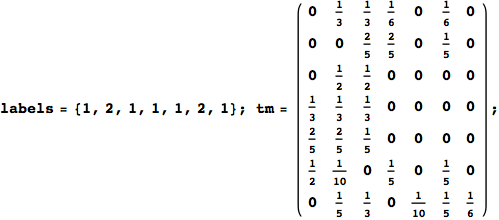
The transition function π is encoded as a n × n matrix of the form {{π(1,1),..., π(1,n)},...,{π(n,1),..., π(n,n)}}.
For instance we can encode the Markov chain M = MC[tm, labels] by defining the variables tm and labels as follows:
In[251]:=

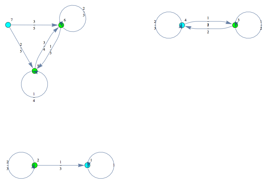
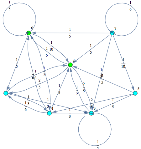
The Markov chain M can be displayed by means of its undelying graph. Labels are displayed using different colors.
In[252]:=

Out[252]=

Another way to encode a transition function is by means of a list of terms of the form Edge[i,π(i,j),j], for 1 ≤ i, j ≤ n.
In[253]:=

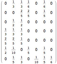
EdgesList is then transformed in a transtition matrix using the function TransitionMatrix[n,EdgeList]
In[254]:=

Out[254]//MatrixForm=

One can check if the encoding corresponds to a well-formed MC by calling MarkovChainQ
In[255]:=

Out[255]=

Given a sequence of Markov chains  they can be joined together using the function JoinMC
In[256]:=

Out[259]=

Run the on-the-fly algorithm
Given a MC M = MC[π,ℓ], a discount factor λ ∈ (0,1], and a list of pairs of states Q, the bisimilarity distance of the pairs in Q can be computed as
In[260]:=

Out[261]=

If one is interested is tracing the computation he can set the option Verbose as True
In[262]:=


Out[262]=

If one is iterestes in computing the distance between all pair of states it suffices to ask for All pairs
In[263]:=

Out[263]=

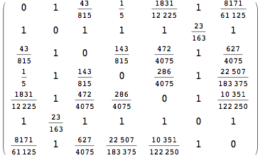
The output is returned as a set of ArrayRules, so that one can easily transform it into a matrix using the function SparseArray
In[264]:=

Out[264]//MatrixForm=

Examples
Example taken from the paper submitted at TACAS 2013
Here we use the MC presented in the paper submitted at TACAS 2013 in order to show most of the features of our on-the-fly algorithm.
In[265]:=

Out[268]=

Let us compute the distance between the state 1 and 4, namely d(1,4)
In[269]:=


Out[269]=

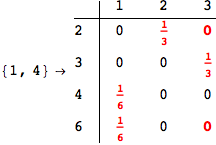
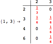
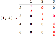
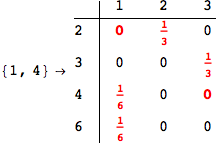
Looking the execution trace we see that during the computation of d(1,4) an over-approximation for the distance d(3,4) is computed.
This happens because the we encountered a coupling that demands d(3,4) for computing an over-approximation of d(1,4).
However, the first improvement of the current coupling makes the computation of d(3,4) no more demanded for d(1,4), so that no further improvement on (3,4) is made.
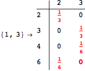
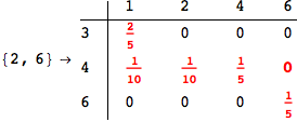
On the other hand, as shown in the execution trace that follows, the exact computation of d(3,4) demands an exact computation of d(1,3), d(1,4) and d(2,6)
In[270]:=


Out[270]=

We have seen that the exact computation of d(3,4) demands for the exact compuatation of d(1,3), d(1,4), d(2,6).
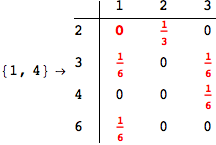
One would claim that if we ask for the exact computation of d(3,4), d(1,4) and d(2,6) the compuatation will do the same steps made for d(3,4).
In some sense this is true, since we will need to compute the same set of distances, however we have seen that the exact computation of d(1,4) does not need an exact compuation of the remaining pairs.
Thus, considering the pair (1,4) before (3,4) will allow us to reduce the size of the linear equation systems computed for d(3,4).
In[271]:=


Out[271]=

Another way to limit the exploration of the MC is to give estimates for some distances. For instance, we have seen that for computing the distance d(3,4) we need to solve exactly
the problem for the pair (2,6). Assume we have an over-approximation of the exact value for d(2,6), we can use this information in order to further reduce the exploration of the MC.
In[272]:=


Out[272]=

Using the estimate  for the distance d(2,6) we considerably reduced the number of steps for computing a good over-approximation for d(3,4).
Unfair Tossing Coins
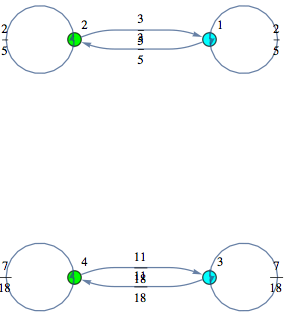
In this example we model two unfair flipping coins.
In[273]:=

Out[275]=

In[276]:=


Out[276]=

The Craps Game
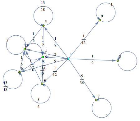
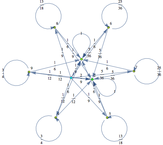
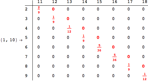
Here we present two different MCs modeling two slightly different versions for the “craps game”. These models have both been taken from the book Principles of Model Checking, Examples 10.4 and 10.23 respectivelty. We compare the two models by means of the distance beteween their initial states.
In[277]:=

In[280]:=

Out[280]=

In[281]:=

In[283]:=

Out[283]=

In[284]:=


Out[284]=

Bisimilarity Distance and Bisimilarity Quotient
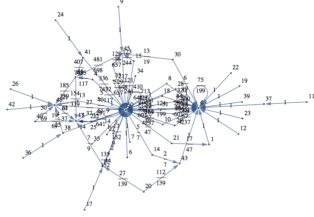
Let M be a (randomly generated) Markov chain with 50 states and outer-degree 2
In[366]:=

Out[368]=

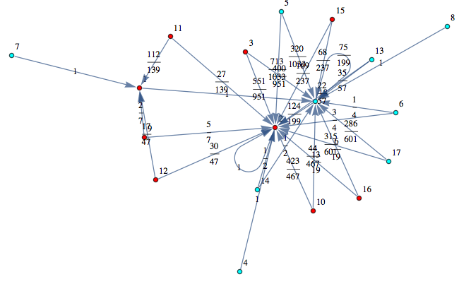
the bisimilarity pseudometric can also be used in order to detect all the bisimilarity classes, i.e. the equivalence classes of the set of state w.r.t probabilistic bisimilarity
In[369]:=

Out[369]=

so that this can be used to construct an MC M’ bisimilar to M with all the states that are bisimilar in M lumped together. M’ is also known as the bisimilar quotient of M.
In[370]:=

Out[370]=

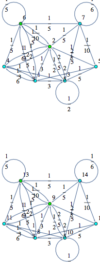
Obvousy, for any MC M, the bisimilarity quotient of two copies of M joined together correspons to M itselfs
In[371]:=

Out[371]=

In[372]:=

Out[372]=

Implementation
Utilities
In[292]:=

In[293]:=

In[294]:=

In[295]:=

In[296]:=

In[297]:=

Labelled Markov Chains (LMCs)
In[298]:=

In[299]:=

In[300]:=

Given a list of edges of the form Edge[s,p,t] indicating that there exists a transition from the state s to t with probability p,
TransitionMatrix[|S|,edgeList] returns the transition matrix π induced by them.
In[302]:=

JoinMC returns a graphical representation of a given Markov chain
In[303]:=

PlotMC returns a graphical representation of a given Markov chain
In[305]:=

Random generation of LMCs
In[307]:=

RandomProbDistr gives a pseudorandom list of rationals  such that
In[308]:=

In[309]:=

In[311]:=

In[312]:=

In[313]:=

Transportation Problem
Given two ε-numbers x and y, EpsilonLeq[x,y] determines if x ≤ y provided that ε → +0.
In[315]:=

In[316]:=

In[317]:=

In[318]:=

In[319]:=

In[320]:=

In[321]:=

In[323]:=

In[324]:=

In[325]:=

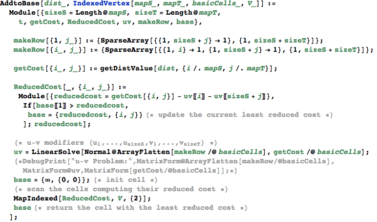
AddtoBase[d, vertex] == {reducedcost, non-basic cell}
returns the non-basic cell which has the minimal reduced cost, if the vertex has no non-basic cells, then it returns {∞, {0,0}}.
In[326]:=

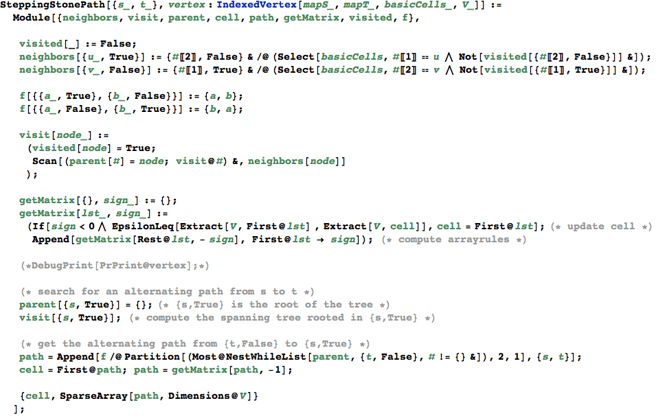
SteppingStone[non-basic cell, vertex] returns the vertex obtained by inserting the given non-basic cell into the base
In[327]:=

In[328]:=

In[329]:=

In[330]:=

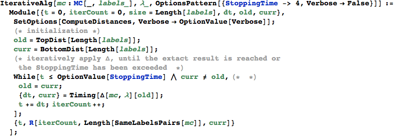
Iterative Algorithm
Given the numer of states |S|, BottomDist[|S|] returns the bottom distance
In[332]:=

In[333]:=

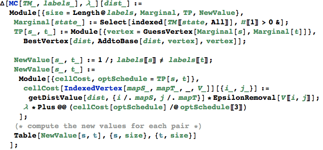
The funtion Δ implements the distance transformer
In[334]:=

In[335]:=

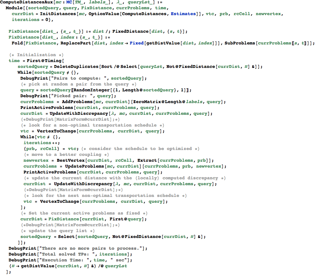
On-the-fly Algorithm for computing Bisimilarity Pseudometric
Given as input an indexed vertex v, SubProblems[v] returns the list of active subproblems. This is simply done by selecting the (non-degenerate) basic cells of ω.
In[336]:=

In[337]:=

In[338]:=

In[339]:=

In[341]:=

In[342]:=

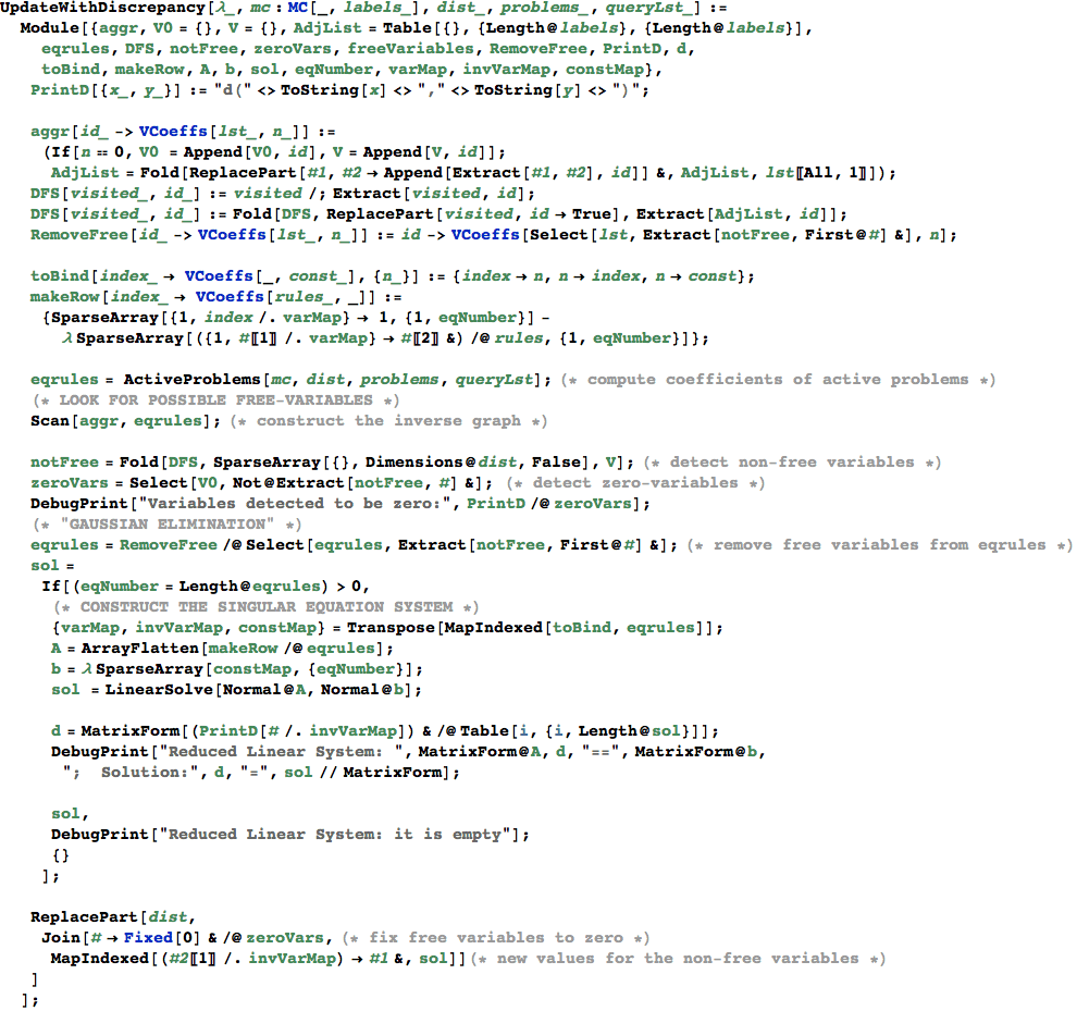
Compute the coefficients  for the given (vertex) schedule
In[343]:=

ActiveProblems maps each active problem to its coefficients 
In[344]:=

In[347]:=

In[350]:=

In[351]:=

In[352]:=

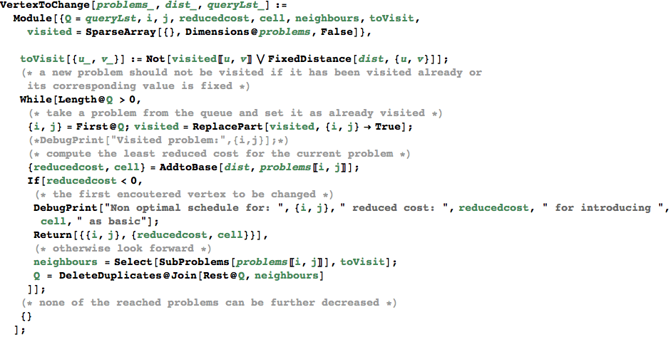
VertexToChange[dist, {s,t}] == {{i,j}, {redCost, nbcell}} if the problem (i,j) can be further minimized, otherwise it returns {}
In[353]:=

In[354]:=

In[362]:=

In[363]:=

Bisimilarity
BisimQuotient[mc] returns an MC with all bisimilar states lumped together
In[364]:=

BisimClasses[mc] returns the quotient w.r.t. bisimilarity
In[365]:=

